Spaced Repetition Algorithm: A Three‐Day Journey from Novice to Expert

I am Jarrett Ye, the principal author of the paper A Stochastic Shortest Path Algorithm for Optimizing Spaced Repetition Scheduling and the paper Optimizing Spaced Repetition Schedule by Capturing the Dynamics of Memory. I currently serve at MaiMemo Inc., where I am chiefly responsible for developing the spaced repetition algorithm within MaiMemo's language learning app. For a detailed account of my academic journey leading to the publication of these papers, please refer to: How did I publish a paper in ACMKDD as an undergraduate?

This tutorial, "Spaced Repetition Algorithms: A Three-Day Journey from Novice to Expert," is adapted from the manuscript I initially prepared for internal presentations at MaiMemo. The objective is to elucidate what exactly spaced repetition algorithms are investigating, and to inspire a new cadre of researchers to contribute to this field and advance the progress of learning technology. Without further ado, let us embark on this intellectual journey.

Preface

From our school days, most students have two simple intuitions:

1. Review information multiple times helps us remember it better.
2. Different memories fade at different rates, not all at once.

These insights raise further questions:

1. How much knowledge have we already forgotten?
2. How quickly are we forgetting them?
3. What is the best way to schedule reviews to minimize forgetting?

In the past, few people have measured these factors or used them to optimize their review schedules. The focus of spaced repetition algorithms is to understand and predict how we remember things and to schedule our reviews accordingly.

In the next three days, we will delve into spaced repetition algorithms from three perspectives:

1. Empirical Algorithms
2. Theoretical Models
3. Latest progresses

Day 1: Exploring Empirical Algorithms

Today we begin our journey by diving into the simplest yet impactful empirical algorithms. We'll uncover the details and the ideas that guide them. But first, let's trace the roots of a term that pervades this field—Spaced Repetition.

Spaced Repetition

For readers new to the subject of spaced repetition, let's learn about the concept of the "forgetting curve."

After we first learn something, whether it's from a book or a class, we start to forget it. This happens gradually, just like the forgetting curve that slopes downward.

The forgetting curve provides an illustration of the way our memory retains knowledge. It exhibits a unique trajectory: in the absence of active review, the decay of memory is initially swift, and slow down over time.

How can we counteract this natural propensity to forget? Let's consider the power of review.

Introducing periodic reviews results in a flattened forgetting curve, indicating a slower decay of memory over time.

In the period following the assimilation of new information, when we undertake a review and characterize our retention with an updated forgetting curve, we find that the curve has become flatter. This indicates that the rate at which we forget has slowed down.

So how should one optimize these review intervals for enhanced memory retention?

Notice the varying lengths of the review intervals? Shorter intervals are used for unfamiliar content, while longer ones are employed for more familiar material, which scatter reviews over different timings in the future. This tactic, known as Spaced Repetition, augment long-term memory retention.

But how effective is it? Let's examine some stats from medical students.

Without Spaced Repetition, students forget 33% of the material after one year and 50% after two years. With Spaced Repetition, however, learning efficiency spikes by 40%.

If Spaced Repetition is so impactful, why hasn't it gained mass adoption?

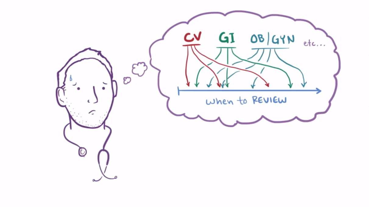
The obstacle lies in the overwhelming volume of knowledge to learn. Each piece of knowledge has its unique forgetting curve, making manual tracking and scheduling a impossible mission.

This introduces the role of spaced repetition algorithms: automating the tracking of memory states and arrange efficient review schedules.

By now, you should have a basic understanding of Spaced Repetition. But questions likely still linger, such as optimal review timing and best practices for efficient Spaced Repetition. The answers to these await in the coming chapters. Let's move on to the heart of the matter!

Review Section

Question	Answer
What aspect of memory does the forgetting curve capture?	The curve describes how knowledge retention decays over time in our memory.
How does memory retention decline when review is not engaged?	It decreases swiftly initially and then slows down.
After a successful review, what distinguishes the new forgetting curve from its predecessor?	The new curve is flatter, indicating a slower rate of forgetting.
What features are specific to the timing of reviews in spaced repetition?	Reviews are distributed over multiple future timings.
How does spaced repetition accommodate content of different familiarity levels?	Shorter intervals are applied for unfamiliar content, while longer ones are set for familiar material.
What function do algorithms serve in spaced repetition?	They automate the tracking of memory states and the arrangement of efficient review schedules.

---

Having delved into the concept of spaced repetition, you may now be pondering this guiding principle:

Shorter intervals are used for unfamiliar content, while longer ones are employed for more familiar material, which scatter reviews over different timings in the future.

What exactly defines these 'short' or 'long' intervals? Furthermore, how can one distinguish between material that is 'familiar' and that which is 'unfamiliar'?

Intuitively, the slower the material is forgotten in our memory, the more familiar it is. And a reasonable interval should minimize our forgetting. But the less we want to forget, the shorter the interval we can deduce from the forgetting curve. The shorter the interval, the higher the frequency of review.

It seems there's an inherent contradiction between the frequency of review and the rate of forgetting—how to reconcile this discrepancy?

Sitting in front of the computer and daydreaming, it seems that no conclusions can be drawn. We still know too little about spaced repetition.

If you were to resolve this conflict, what would you need to continue to learn? What kind of experiment would you design? Keep thinking about them, and even better, write them down!

Let's take a look at how the creator of the first computational spaced repetition algorithm set out on his journey in the exploration of memory.

SM-0

In 1985, a young college student named Peter Wozniak (aka Woz) was struggling with the problem of forgetting:

The above image shows a page from his vocabulary notebook, which contained 2,794 words spread across 79 pages. Each page had about 40 pairs of English-Polish words. Managing their review was a headache for Wozniak. At first, he didn't have a systematic plan for reviewing the words; he just reviewed whatever he had time for. But he did something crucial: he kept track of when he reviewed and how many words he forgot, allowing him to measure his progress.

He compiled a year's worth of review data and discovered that his rate of forgetting ranged between 40% and 60%. This was unacceptable to him. He needed a reasonable study schedule that would lower his forgetting rate without overwhelming him with reviews. To find an optimal review interval, he commenced his own memory experiments.

Wozniak wanted to find the longest possible time between reviews, while keeping the forgetting rate under 5%.

Here are the details about his experiment:

Materials: Five pages of English-Polish vocabulary, each with 40 word pairs.

Initial Learning: Memorize all 5 pages of material. The specific operation is: look at the English, recall the Polish, and then check whether the recall is correct. If the recall is correct, eliminate the word pair from this phase. If the recall fails, try to recall it later until all the memories are correct.

Initial Review: A one-day interval was employed for the first review, based on Woz's previous review experience.

The ensuing key phases—A, B, and C—revealed the following:

Phase A: Woz reviewed five pages of notes at intervals of 2, 4, 6, 8, and 10 days. The resulting forgetting rates were 0%, 0%, 0%, 1%, and 17%, respectively. He determined that a 7-day interval was optimal for the second review.

Phase B: A new set of five pages was reviewed after 1 day for the first time, and then after 7 days for the second time. For the third review, the intervals were 6, 8, 11, 13, and 16 days, with forgetting rates of 3%, 0%, 0%, 0%, and 1%. Wozniak selected a 16-day interval for the third review.

Phase C: Another fresh set of five pages was reviewed at 1, 7, and 16-day intervals for the first three reviews. For the fourth review, the intervals were 20, 24, 28, 33, and 38 days, with forgetting rates of 0%, 3%, 5%, 3%, and 0%. Wozniak opted for a 35-day interval for the fourth review.

Subsequently, Woz conducted experiments to identify the optimal interval for the fifth review. However, the time required for each successive phase was approximately double that of the preceding one. Ultimately, he formalized the SM-0 algorithm on paper.

• I(1) = 1 day
• I(2) = 7 days
• I(3) = 16 days
• I(4) = 35 days
• for i>4: I(i) = I(i-1) * 2
• Words forgotten in first four reviews were moved to a new page and cycled back into repetition along with new materials.

In this context, $I(i)$ denotes the interval employed for the $i^{th}$ review. The interval for the fifth repetition was set to be twice that of the preceding one, a stipulation grounded in intuitive assumptions. Over the two years of utilizing the SM-0 algorithm, Woz collected sufficient data to corroborate the validity and accuracy of this hypothesis.

The goal of the SM-0 Algorithm was clear: to extend the review interval as much as possible while minimizing the rate of memory decay. Its limitations were evident as well, namely its inability to track memory retention at a granular level.

Nonetheless, the significance of the SM-0 Algorithm was far-reaching. With the acquisition of his first computer in 1986, Woz simulated the model and drew two key conclusions:

• Total knowledge retention could increase over time.
• The learning rate remained relatively stable in the long term.

These insights proved that the algorithm could reconcile the tension between memory retention and the frequency of review. Woz realized that spaced repetition didn't have to mire learners in a cycle of endless review, thereby inspiring him to continue refining spaced repetition algorithms.

Review Section

Questions	Answers
Which two factors did Woz consider for determining optimal review intervals?	Interval duration, which is linked to the frequency of review, and the rate of memory decay, associated with memory retention.
Why did Woz use new materials each time he sought to establish a new review interval in his experiments?	To ensure uniformity in the intervals of prior reviews, thus controlling for variables.
What is the primary limitation of the SM-0 Algorithm?	It uses a page of notes as the unit for review, making it unsuitable for tracking memory retention at a more granular level.

SM-2

Though the SM-0 algorithm displayed initial efficacy, several issues prompted Wozniak to seek refinements:

1. If a word is forgotten during the first review (after 1 day), it will be easier to forget again in the second and third reviews (after 7 and 16 days) compared to words that were not forgotten before.

2. Pages of new notes made up of words forgotten after the fourth review have a higher forgetfulness rate under the same review schedule.

The first finding made him realize that reviewing doesn't always make him more familiar with the material. Forgotten stuff gets even more unfamiliar, and the speed of forgetting doesn't slow down. If he keeps reviewing these words with longer gaps like the rest on the same note page, it won't work well.

The second finding made him see that not all material is equally hard. Different difficulty levels should have different review gaps.

Consequently, in 1987, armed with his initial personal computer, Woz utilized his two-year record and insights from the SM-0 algorithm to craft the SM-2 algorithm.

The details about SM-2:

• Break down the information you want to remember into small question-answer pairs.
• Use the following gaps (in days) to repeat each question-answer pair:

  • $I(1) = 1$

  • $I(2) = 6$

  • For $n > 2$, $I(n) = I(n-1) \times EF$

    • $EF$—the Ease Factor, with an initial value of 2.5
    • After each review, $\text{newEF} = EF + (0.1 - (5-q) \times (0.08 + (5-q) \times 0.02))$
      • $\text{newEF}$—the post-review updated value of the Ease Factor
      • $q$—the quality grades of review, ranging from 0 - 5. If it's >= 3, it means the learner remembered, and if it's < 3, the learner forgot.

  • If the learner forgets, the interval for the question-answer pair will be reset to $I(1)$ with the the same EF.

The SM-2 algorithm adds the review feedback into how often you review the question-answer pairs. This feedback kinda shows how hard or easy they are. The lower the EF, the smaller the interval multiple factor.

The SM-2 algorithm still relies on Woz's own experimental data, but two main updates make it a popular spaced repetition algorithm today:

1. It breaks down the notes page into smaller question-answer pairs. This lets the review schedule be super specific to each pair and separates out the hard and easy stuff sooner.

2. It uses an "Ease Factor" and grades. So, the algorithm can modify the learner's future reviews based on how well the learn remembers.

Review Section

Questions	Answers
Why shouldn't we set a longer interval for stuff we forgot during review?	The speed of forgetting for those things doesn't slow down.
What shows that some stuff is harder to remember than others?	The pages with stuff that got forgotten have a higher rate of being forgotten again.
What is the functional utility of incorporating an "Ease Factor" and "Quality Grade" into the SM-2 algorithm?	This enables the algorithm to dynamically adjust future review intervals based on user performance.
What are the advantages of breaking down note pages into smaller parts for review?	It lets the algorithm sort out the easier and harder stuff sooner for when to review them next.

SM-4

The primary objective of SM-4 is to address the shortcomings in adaptability found within its predecessor, the SM-2 algorithm. While SM-2 has the capacity to tune review schedules for individual flashcards based on ease factors and recall grades, these adjustments are made in isolation, without regard to prior alterations made to other cards.

In other words, each flashcard is treated as an independent entity in SM-2, leaving the algorithm perpetually uninformed about the user's overall learning process, regardless of the quantity of cards reviewed. To overcome this, SM-4 introduces an Optimal Interval Matrix, replacing the existing formulae used for interval calculations:

The matrix above is called the Optimal Interval (OI) matrix. It has rows for how easy stuff is and columns for how many times you've seen it. It starts the same as SM-2, using the same formulas to decide how long to wait before looking at a card again.

To make new cards learn from what happened with old cards, the OI matrix keeps changing as the learner reviews. The main idea is: if the OI matrix says to wait X days and the learner actually waits X+Y days and still remembers with a high grade, then the OI value should be changed to something between X and X+Y.

The reason for this is simple: if the learner can remember something after waiting X+Y days and get a good score, then the old OI value was probably too short. Why not make it longer?

This naive idea allows SM-4 to be the first algorithm capable of making holistic adjustments based on the learner's experience. But, it didn't work as well as hoped. The reasons are simple:

1. Each review only changes one entry of the matrix, so it takes too long to really make the OI matrix better.
2. For longer review interval, it takes a long time to make them stable.

To address these issues, the SM-5 algorithm was designed. But I won't go into details here because of space limits.

Review Section

Question	Answer
What accounts for the limited adaptability of SM-2?	Adjustments are made to each flashcard in isolation, precluding the sharing of experiential insights.
What components does SM-4 introduce to enhance adaptability?	Optimal Interval Matrix and dynamic interval-adjustment rules.
What is the underlying principle for interval adjustments in SM-4?	If the learner exhibits proficient recall over extended intervals, the original interval should be longer, and vice versa.

Summary

Invented in 1885, the Forgetting Curve shows how we remember and forget. Fast-forward to 1985, the computational spaced repetition aimed to find the optimal review schedule. This section has outlined the developmental progression of empirically based algorithms:

• SM-0 gathered experimental data to determine the best review intervals for a given individual and a specific type of material (Woz defined what "best" means here).
• SM-2 digitalized the algorithm for computer applications, introducing more granular card level and incorporating adaptive ease factors and recall grades.
• SM-4 further enhanced the adaptability of the algorithm for a diverse range of learners, introducing the Optimal Interval Matrix along with rules for adjusting the intervals.

While empirical algorithms offer a valuable lens through which to understand Spaced Repetition, it's really hard to make it better without a systematic theoretical underpinning. So, hang on! We're speeding up and diving into the theory part next!

Day 2: Understanding Theoretical Models

Memory algorithms sound like a theoretical study, but I've spent a lot of space on empirical algorithms. Why?

Because memory algorithms are an artificial science. Although memory is a natural phenomenon of human physiology, regular review to enhance memory is a strategy constructed by humans ourselves.

Without the foundational support of empirical approaches, any theoretical discourse would be without merit. The gut feelings we have about theory come from real-world experience.

So, the theories we'll talk about next will also start from what we've learned by doing. No building castles on sand here!

Two Components of Memory

Here's a question to think about: What factors would you consider when describing the state of something in your memory?

Before Robert A. Bjork, many researchers used memory strength to talk about how well people remembered something.

Do you think memory strength is enough to describe how well you remember something?

Let's revisit the Forgetting Curve for a moment:

First and foremost, Memory Retention (Recall Probability) clearly emerges as a pivotal variable in characterizing the state of one's memory. Derived from our quotidian experiences, forgetting often manifests as a stochastic phenomenon. No one can unequivocally assert that a word memorized today will be retained ten days hence or forgotten twenty days later.

Is recall probability sufficient for description? Imagine drawing a horizontal line across these Forgetting Curves; each curve will intersect at a point with identical recall probabilities. Have you noticed that recall probability alone seems insufficient for differentiating the conditions at these intersections?

Precisely, solely relying on recall probability does not allow us to distinguish the rate of forgetting associated with different materials. While this rate should certainly be factored into the description of memory states, it's a variable that changes with time. Can we depict it through a temporal-independent metric?

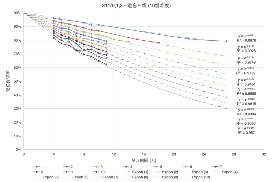
To address this quandary, we must delve into the mathematical properties of the forgetting curve—a task that necessitates the gathering of extensive data to plot the curve. The data, in this tutorial, is sourced from an open dataset created from language learning application MaiMemo.

From the figure above, we find that the forgetting curve approximates a negative exponential function with a base of $e$. The rate of forgetting can be captured by the corresponding decay constant of this function.

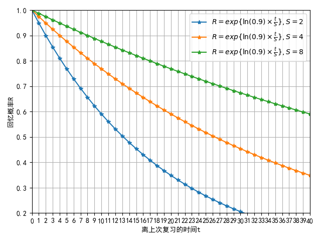
Considering that this decay constant is difficult to relate to the function image, we tend to transform this decay constant to obtain a fitting formula for the forgetting curve:

$$ \begin{aligned} R = \exp\left[\frac{t \ln{0.9}}{S}\right] \end{aligned} $$

In this equation, $R$ symbolizes the Probability of Recall, $S$ denotes the Memory Stability, and $t$ accounts for the time that has elapsed since the last review.

The correlation between $S$ and the shape of forgetting curve is displayed in the following figure:

The notion of "Memory Stability," $S$, corresponds precisely to the duration required for the "Probability of Recall," $R$, to decline from 100% to 90%. (In alternative scholarly literature, a 50% benchmark is often employed, in which case the stability is referred to as the memory's half-life.)

The two strengths of memory proposed by Bjork's - retrieval strength and storage strength - corresponds precisely to recall probability and memory stability.

The equation embodies three distinct properties:

1. When $t=0$, $R=100%$, signifying that upon immediate review, the process of forgetting has not yet been initiated, rendering the Probability of Recall at a maximal level.

2. As $t$ approaches infinity, $R$ converges toward zero, indicating that if you never review something, you will forget almost all of them.

3. The first derivative of the negative exponential function is diminishing, aligning with the empirical observation that forgetting is fast initially and slow down subsequently.

Thus, we have delineated two integral components of memory, but seems like something's missing.

The Probability of Recall quantifies the extent of forgetting, while Memory Stability characterizes the rate of forgetting; what else is not described?

Well, the moment when the shape of forgetting curve changes! The memory stability changes, and it doesn't only rely on the Probability of Recall at review and its previous Memory Stability.

Is there evidence to substantiate this claim? Think about the first time you learn something: your memory stability and probability of recall are both zero. But after you learn it, your probability of recall is 100%, and the memory stability depends on a certain property of the stuff you just learned.

Basically, the thing you're trying to remember itself has some features that can affect your memory. Intuitively, this variable is the difficulty of material.

With this variable of difficulty added, we now have a three-components model to describe memory.

Review Section

Question	Answer
Why can't a single variable of memory strength adequately describe the state of memory?	A single variable is insufficient because the forgetting curve encompasses both retention levels and the rate of forgetting.
What variable measures the degree of memory retention?	Recall Probability
Which function can approximate the forgetting curve?	Exponential Function
What variable measures the speed of forgetting?	Decay Constant
What is the practical implication of memory stability?	The time required for the recall probability to decline from 100% to a predetermined percentage, often 90%.

The Three Component Model of Memory

Let us delve directly into the terms:

• Memory Stability: The duration required for the probability of recall for a particular memory to decline from 100% to 90%.
• Memory Retrievability: The probability of recalling a specific memory at a given moment.
• Memory Difficulty: The inherent complexity associated with a particular memory.

The difference between Memory Retrievability and Memory Retention: the former pertains to the recall probability of a singular memory, whereas the latter refers to the average recall probability for a population of memories.

With above terms, one can define the retrievability of any given memory at time $t$ following $n$ successful recall:

$$ R_n(t) = \exp\left[\cfrac{t\ln{0.9}}{S_n}\right] $$

By transforming $S_n$ into the inter-review interval, this equation bridges the interval between spaced repetition algorithms and memory models:

$$ R_n(t) = \exp\left[\cfrac{t\ln{0.9}}{I_1\prod\limits_{i=2}^{n}C_i}\right] $$

Where:

• $I_1$ denotes the interval prior to the first review.
• $C_i$ represents the ratio between the $i$-th review interval and the preceding $i-1$-th review interval.

The objective of spaced repetition algorithms is to accurately compute $I_1$ and $C_i$, thereby ascertaining the stability of memory across varied students, materials, and review schedules, which facilitates the optimization of review intervals.

To recapitulate, both SM-0 and SM-2 algorithms have an $I_i$ of one day. In SM-0, $C_i$ is a predetermined constant, whereas in SM-2, $C_i$ is a variable Ease Factor (EF) that adjusts in response to user input. It is imperative to note that each card's $C_i$ is independent of others. SM-4 attempts to break through this independence, and has been continuously improved on SM-5 and subsequent algorithms.

The question is, what is the relationship between $C_i$ and the three-variable of memory?

One could ponder this by thinking how the state of memory updates during each review.

Below are some empirical observations of Woz, corroborated by data from vocabulary learning platforms like MaiMemo:

• Impact of Memory Stability: A higher $S$ yields a smaller $C_i$. This signifies that as memory becomes more stable, its subsequent stabilization becomes increasingly hard.
• Impact of Memory Retrievability: A lower $R$ results in a larger $C_i$. This implies that a lower probability of recall leads to greater post-recall stability.
• Impact of Memory Difficulty: A higher $D$ engenders a smaller $C_i$. Essentially, greater complexity in the material leads to a smaller increment in stability.

Due to the multifarious factors at play, $C_i$ is hard to calculate. SuperMemo employs a multi-dimensional matrix to represent $C_i$ as a multivariable function and adjusts the matrix values during the user's learning journey to approximate real-world scenarios.

For the sake of subsequent discourse, we shall adopt SM-17's naming for $C_i$: Stability Increase (SInc). The term implies that $C_i$ represents the multiple in memory stability before and after review.

Let us now delve into a more detailed exposition of Stability Increase.

Review Section

Question	Answer
Which three variables are encapsulated in the three-variable model of memory?	Memory Stability, Memory Retrievability, and Memory Difficulty
What differentiates Memory Retrievability from Memory Retention Rate?	The former pertains to the attributes of individual memories, whereas the latter refers to the general attributes of the population of memories.
What two parameters serve as the linchpin connecting the three-variable model of memory and memory algorithms?	The initial review interval $I_1$ and the ratio $C_i$ between successive intervals.
What nomenclature is applied to $C_i$?	Stability Increase

Memory Stability Increase

In this chapter, we momentarily set aside the influence of memory difficulty to focus on the intricate relationship between memory stability increase, stability, and retrievability.

Data for the ensuing analysis is collected from SuperMemo users and scrutinized by Woz through controlled variables and linear regression techniques.

Dependence of stability increase on S

Upon investigating the Stability Increase (SInc) matrix, it became evident that for a given level of Retrievability (R), the function of SInc with respect to Stability (S) can be aptly characterized by a negative power function.

By taking the logarithm of both Stability Augmentation (Y-axis) and Stability (X-axis), the following curve is attained:

This corroborates our prior qualitative conclusion, "As S increases, $C_i$ decreases," and provides a more nuanced delineation of its functional properties.

Dependence of stability increase on R

As predicted by the spacing effect, Stability Increase (SInc) is more pronounced when Retrievability (R) is low. After analyzing multiple datasets, it was observed that SInc demonstrates exponential growth as R diminishes—a surge that surpasses initial expectations, thereby further substantiating the spacing effect.

Upon logarithmically transforming Retrievability (X-axis), the following curve is achieved:

Intriguingly, SInc may fall below one when R is at 100%. Molecular-level research suggests an increase in memory instability during review sessions, thereby corroborating once more that rote repetition not only squanders time but also impairs memory.

Conclusions derived from stability increase formula

In light of the aforementioned fundamental laws, one can derive an array of compelling conclusions through varied perspectives and combinatorial approaches.

Linear increase in value of review over time

As time (t) increases, Retrievability (R) exponentially diminishes, while Stability Increase (SInc) conversely exhibits an exponential ascent. These two exponents counterbalance each other, yielding an approximately linear trajectory.

Expected increase in memory stability

Optimization in learning encompasses diverse benchmarks; one could tailor strategies for specific retention rates or aim to maximize memory stability. In either scenario, comprehending the anticipated stability augmentation proves advantageous.

We define the expected stability augmentation as:

$$ E(SInc) = SInc \times R $$

This equation divulges a startling revelation: the apex of anticipated stability augmentation occurs when the retention rate resides between 30% and 40%.

It's crucial to note that maximal expected stability increase does not necessarily equate to the swiftest learning velocity. For the most efficacious review schedule, refer to the forthcoming SSP-MMC algorithm.

Review Section

Question	Answer
What mathematical function describes the relationship between stability increase and memory stability?	Negative power function
What mathematical function describes the relationship between stability increase and memory retrievability?	Exponential function

Memory Complexity

Memory stability during spaced repetition is contingent upon the quality of review, termed here as memory complexity. For efficacious review sessions, knowledge associations must remain simplistic—even if the knowledge itself is intricate. Flashcards can encapsulate complex knowledge architectures, yet individual flashcards ought to remain atomic.

In 2005, we formulated an equation to describe the review of composite memories. We observed that the stability of a composite memory behaves akin to resistance in a circuit; parallel resistance allows greater electrical current to pass through. (*Note: Composite is used in lieu of complex to emphasize its composed nature of simpler elements.)

Composite knowledge yields two primary ramifications:

• Augmentation in interference from additional information fragments
• Difficulty in uniformly stimulating the sub-components of the memory during review

Suppose we possess a composite flashcard that requires the memorization of two fill-in-the-blank fields. Assume both blanks are equally challenging to remember. Hence, the retrievability of the composite memory is the product of the retrievabilities of its sub-memories.

$$ R = R_a \times R_b $$

Inserting this into the decay curve equation,

$$ R = e^{ \frac{t \ln 0.9}{S_a}} \times e^{ \frac{t \ln 0.9}{S_b}} = e^{ \frac{t \ln 0.9}{S}} $$

Here, $S$ denotes the stability of this composite memory. We can deduce:

$$ \frac{t \ln 0.9}{S} = \frac{t \ln 0.9}{S_a} + \frac{t \ln 0.9}{S_b} $$

Leading to,

$$ S = \frac{S_a \times S_b}{S_a + S_b} $$

Remarkably, the stability of a composite memory will be inferior to the stabilities of its constituent memories. Based on this derivation, the stabilities of the two sub-memories will converge towards the stability of the more challenging sub-memory.

As complexity ascends beyond a certain threshold, the establishment of enduring memory stability becomes unattainable. Succinctly put, the only alternative to engraining an entire tome into one's memory is ceaseless rereading—a futile endeavor.

Review Section

Question	Answer
What is the relationship between the retrievability $R$ of a composite memory and the retrievabilities $R_a, R_b$ of its constituent memories?	$R = R_a \times R_b$; the retrievability of a composite memory is the product of the retrievabilities of its individual components.
What is the comparative magnitude between the stability $S$ of a composite memory and the stabilities $S_a, S_b$ of its constituent memories?	The stability of a composite memory is inferior to the stabilities of its individual components.
How does the stability of a composite memory change as the number of its constituent memories increases?	It progressively diminishes, asymptotically approaching zero.

Day 3: Following Latest Progresses

After learning some theories of memory, it's time to put them into practice (You've learned 1+1=2, now let's solve this infinite series together, XD). The upcoming advancements will introduce how MaiMemo applies these memory theories, develops its own spaced repetition algorithms, and improves users' memory efficiency.

There will be no review section next, and the difficulty will increase sharply, so be prepared!

Collect Data

Data is the lifeblood of memory algorithms. Without data, even the most skilled person cannot achieve anything. Collecting appropriate, comprehensive, and accurate data will determine the upper limit of spaced repetition algorithms.

To accurately depict a learner's memory states, we need to define the basic behavior of memory. Let's think about it: what are the important attributes of a memory behavior?

The most basic elements are easy to think of: who (the subject), when (time), and what (memory). For memory, we can further explore: what was remembered (content), how well it was remembered (response), and how long it took (cost), etc.

Taking these attributes into consideration, we can use a tuple to record a memory behavior event:

$$ e := (\text{user}, \text{item}, \text{time}, \text{response}, \text{cost}) $$

This event records a user's response and cost for a particular item at a certain time. For example:

$$ e := (\text{Jarrett}, \text{apple}, \text{2022-04-01 12:00:01}, \text{Forgotten}, \text{5s}) $$

That is: Jarrett reviewed the word "apple" at 12:00:01 on April 1st, 2022, forgot it, and cost 5 seconds.

With the basic definition of memory behavior events, we can extract and calculate more information of interest based on this foundation.

For example, in spaced repetition, the interval between two repetitions is essential information. Using the memory behavior events mentioned above, we can group event data by user and item, sort by time, and then subtract the time of two adjacent events to obtain the interval. Generally, to save calculation steps, the interval can be directly recorded in the event. Although this causes storage redundancy, it saves computational resources.

In addition to time intervals, the historical sequences of feedback and intervals are also important features. For example, "forgot, remembered, remembered, remembered" and "1 day, 3 days, 6 days, 10 days" can reflect a memory behavior's independent history more comprehensively and can be directly recorded in memory behavior events:

$$ e_{i} := (\text{user}, \text{item}, \boldsymbol{\Delta t_{1:i-1}}, \boldsymbol{r_{1:i-1}}, \Delta t_i, r_i) $$

If you are interested in the data, you can download the open-source dataset from MaiMemo and analyze it yourself.

The DSR Model

Now that we have the data, how can we use it? Reviewing the three-variable memory model from Day 2, what we want to know are the various attributes of memory states, which our current data collection does not include. Therefore, the goal of this section is to convert memory behavior data into memory states and their transition relationships.

Memory States

The three letters in the DSR model correspond to difficulty, stability, and retrievability. Let's start with retrievability. Retrievability reflects the probability of recalling a memory at a certain moment, but memory behavior events are the results after recalling. In probabilistic terms, memory behavior is a single random experiment with only two possible outcomes, and its success probability equals retrievability.

Therefore, the most straightforward method to measure retrievability is to perform countless independent experiments on the same memory and then count the frequency of successful recall. However, this method is infeasible in practice. Because experimenting with memory will change its state, we cannot act as an observer and measure memory without affecting it. (Note: With the current level of neuroscience, it is still impossible to measure memory states at the neural level, so this approach is also unavailable for now.)

So, are we out of options? Currently, there are two compromise measurement methods: (1) Ignore the differences in memory materials: SuperMemo and Anki both belong to this category; (2) Ignore the differences among learners: MaiMemo belongs to this category. (Note: This has been considered now, but it was not when I started writing this paragraph. However, it does not matter, as it will not affect the understanding of the following content.)

Ignoring the differences in memory materials means that when measuring retrievability, we collect data with the same attributes except for the memory materials. Although it is impossible to perform multiple independent experiments on one learner and one material, it can be done with one learner and multiple materials. On the other hand, ignoring the differences among learners involves collecting data from multiple learners with the same material.

Considering the sufficient amount of data in MaiMemo, this section will only introduce the measurement method that ignores learner differences. After ignoring them, we can aggregate to obtain a new group of memory behavior events:

$$ e_{i} := (item, \boldsymbol{\Delta t_{1:i-1}}, \boldsymbol{r_{1:i-1}}, \Delta t_i, p_i, N) $$

Here, N is the number of learners who have memorized the same material and have the same historical behavior. Retrievability $p=\frac{n_{r=1}}{N}$ is the proportion of successful recall among these learners. When $N$ is large enough, the ratio $n_{r=1}/N$ approaches the true retrievability.

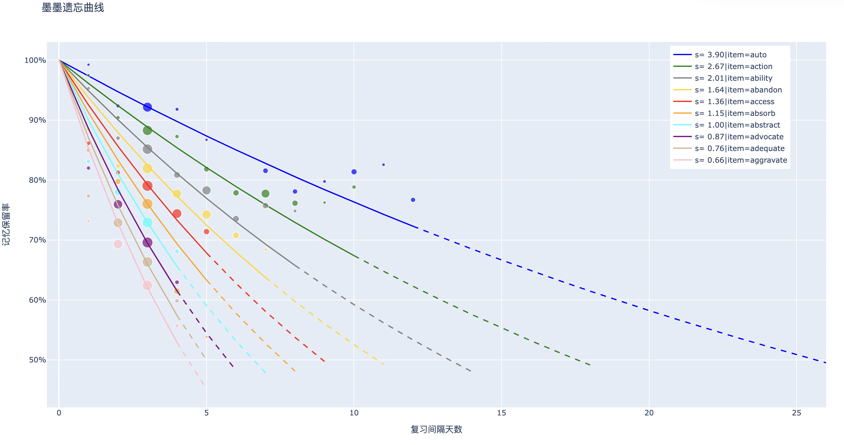
After solving the retrievability issue, the stability can be easily addressed. The method to measure stability is the forgetting curve. Based on the collected data, an exponential function can be used to regress and calculate the stability of memory behavior event groups with the same $(item, \boldsymbol{\Delta t_{1:i-1}}, \boldsymbol{r_{1:i-1}})$.

The scatter plot coordinates are $(\Delta t_i , p_i)$, with relative size as $\log N$. The curve is the fitted forgetting curve.

Finally, it's time to tackle the difficulty. How can we derive the difficulty from memory data? Let's start with a simple thought experiment. Suppose a group of learners memorize the words apple and accelerate for the first time. How can we use memory behavior data to distinguish the difficulty of the two words?

The simplest method is to test immediately the next day, record the memory behavior data, and see which word has a higher recall proportion. Based on this starting point, we can replace the recall proportion on the second day with the stability after the first memory.

That is to say, the stability after the first memory can reflect the difficulty. However, there is no unified standard for using the stability after the first memory to divide the difficulty. There is also no consensus on the best way to divide it. As an introductory material, this article will not discuss it in detail.

State Transition

So far, we can transform memory behavior data into memory states: $$ (item, \boldsymbol{\Delta t_{1:i-1}}, \boldsymbol{r_{1:i-1}} , \Delta t_i , p_i, N) => (D_i, S_i, R_i) $$

Next, we can start describing the transition relationship between states. What is the relationship between $(D_i, S_i, R_i)$ and $t$, $r$ after reviewing in $\Delta t$ days, with the recall result being $r$, and obtaining the new memory state $(D_{i+1}, S_{i+1}, R_{i+1})$?

First, we still need to organize the memory state data into a form suitable for analysis:

$$ (D_i, S_i, R_i, \Delta t, r, D_{i+1}, S_{i+1}, R_{i+1}) $$

Here, $R_{i+1}$ will immediately reach 100% after review, so it can be ignored during the analysis. Also, between $R_i$, $\Delta t$, and $S_i$, knowing two can help determine the other, so we can ignore $\Delta t$.

In the end, the state transition data we need to analyze is as follows:

$$ (D_i, S_i, R_i, r, D_{i+1}, S_{i+1}) $$

And $\cfrac{S_{i+1}}{S_i}=SInc$, which can refer to the patterns we mentioned in the memory stability growth chapter:

$$ SInc = a S^{-b} $$

$$ SInc = c e^{-d R} $$

We can obtain the relationship formula (the influence of difficulty D is omitted here):

$$ S_{i+1} = S_{i} \cdot a S_{i}^{-b} e^{-c R_i}\textrm{(if r = 1)} $$

According to the above formula, we can predict the memory state $(D_{i+1}, S_{i+1})$ of learners after each successful recall. The feedback forgetting is the same, and it can be described by another set of state transition equations.

Spaced Repetition System Simulation

With the DSR memory model, we can simulate memory states under any review schedules. So, how should we simulate it specifically? We need to start from the perspective of how ordinary people use spaced repetition software in reality.

Suppose Jarrett needs to prepare for the GRE in four months and needs to use spaced repetition to memorize the English words in the exam syllabus. However, time must also be allocated to prepare for other subjects.

From the above sentence, there are two obvious constraints: the number of days before the deadline and daily learning time. The Spaced Repetition System (SRS) simulator needs to take these two constraints into consideration, and this also highlights the two dimensions of SRS simulation: by day and in day. In addition, the number of syllabus words is limited, so the SRS simulation also has a finite set of cards, from which learners select materials for learning and review every day. The arrangement of review tasks is managed by the spaced repetition scheduling algorithm. To sum up, SRS simulation requires:

1. Material set
2. Learner
3. Scheduler
4. Simulation duration (in day + by day)

The learner can be simulated using the DSR model, providing feedback and memory state for each review. The scheduler can be SM-2, Leitner System, or any other algorithm for scheduling reviews. The simulation duration and material set need to be set according to the situation to be simulated.

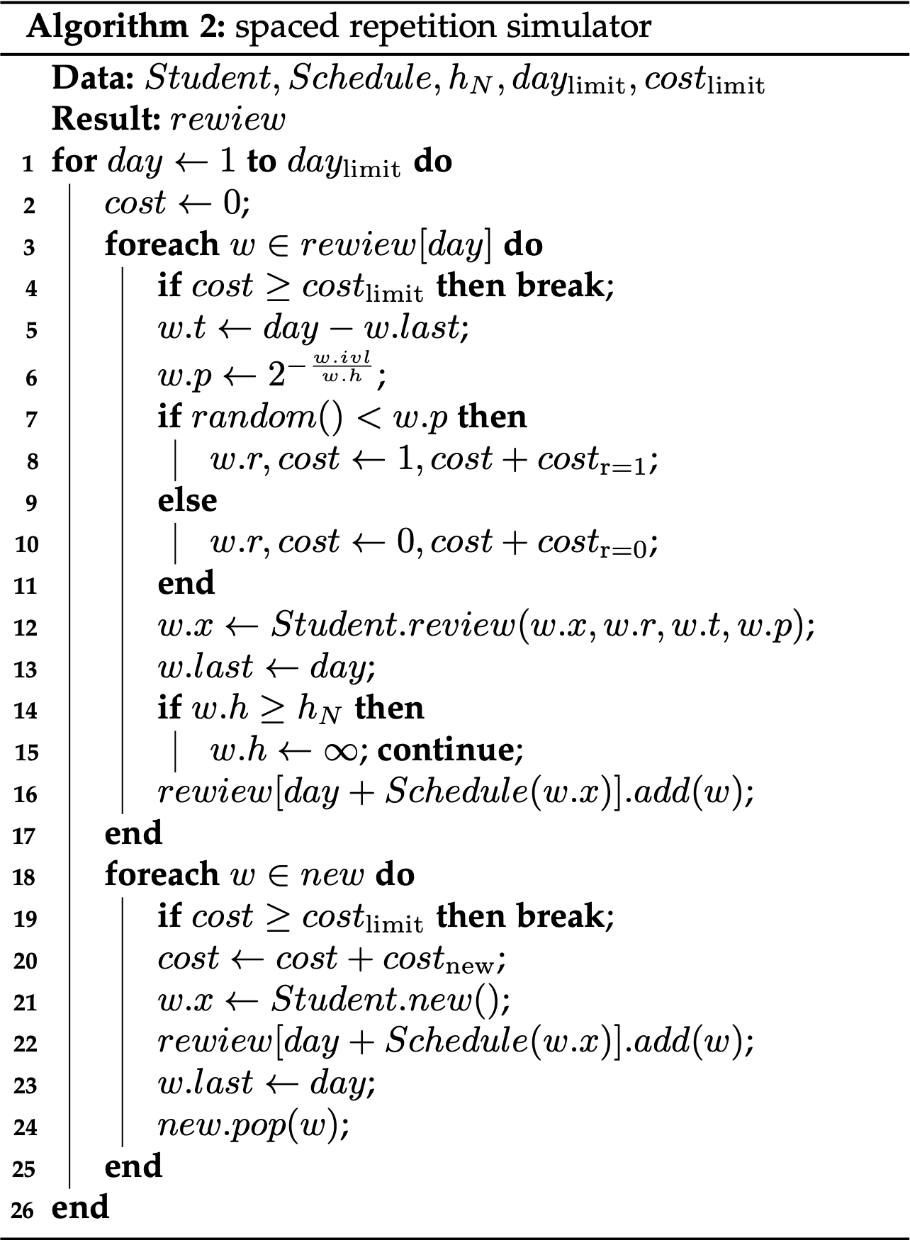
Then, we will design a specific simulation process based on the two dimensions of SRS simulation. Obviously, we need to simulate day by day into the future in chronological order, and the simulation of each day is composed of feedback from card by card. Therefore, the SRS simulation can consist of two loops: the outer loop represents the current simulated date, and the inner loop represents the current simulated card. In the inner loop, we need to specify the time spent on each review, and when the accumulated time exceeds the daily learning time limit, the loop is automatically exited, ready to enter the next day.

Here is the pseudocode for SRS Simulation:

The pertinent Python code has been open-sourced on GitHub for readers who are intrigued enough to delve into the source code: L-M-Sherlock/space_repetition_simulators: Spaced Repetition Simulators (github.com)

SSP-MMC Algorithm

Having discussed the DSR model and SRS simulation, we can now predict learners' memory states and memory situations under given review schedules, but we still haven't answered our ultimate question: What kind of review schedules is the most efficient? How to find the optimal review schedule? The SSP-MMC algorithm solves this problem from the perspective of optimal control.

SSP-MMC is an acronym for Stochastic Shortest Path and Minimize Memorization Cost, encapsulating both the mathematical toolkit and the optimization objective underpinning the algorithm. The ensuing discourse is adapted from my graduate thesis, "Research on Review Scheduling Algorithms Based on LSTM and Spaced Repetition Models," and the conference paper A Stochastic Shortest Path Algorithm for Optimizing Spaced Repetition Scheduling.

Problem Setup

The purpose of the spaced repetition method is to help learners form long-term memory efficiently. Whereas the memory stability measures the storage strength of long-term memory, the number of repetitions and the time spent per repetition reflect the cost of memory. Therefore, the goal of spaced repetition scheduling optimization can be formulated as either getting as much material as possible to reach the target stability within a given memory cost constraint or getting a certain amount of memorized material to reach the target stability at minimal memory cost. Among them, the latter problem can be simplified as how to make one memory material reach the target stability at the minimum memory cost (MMC).

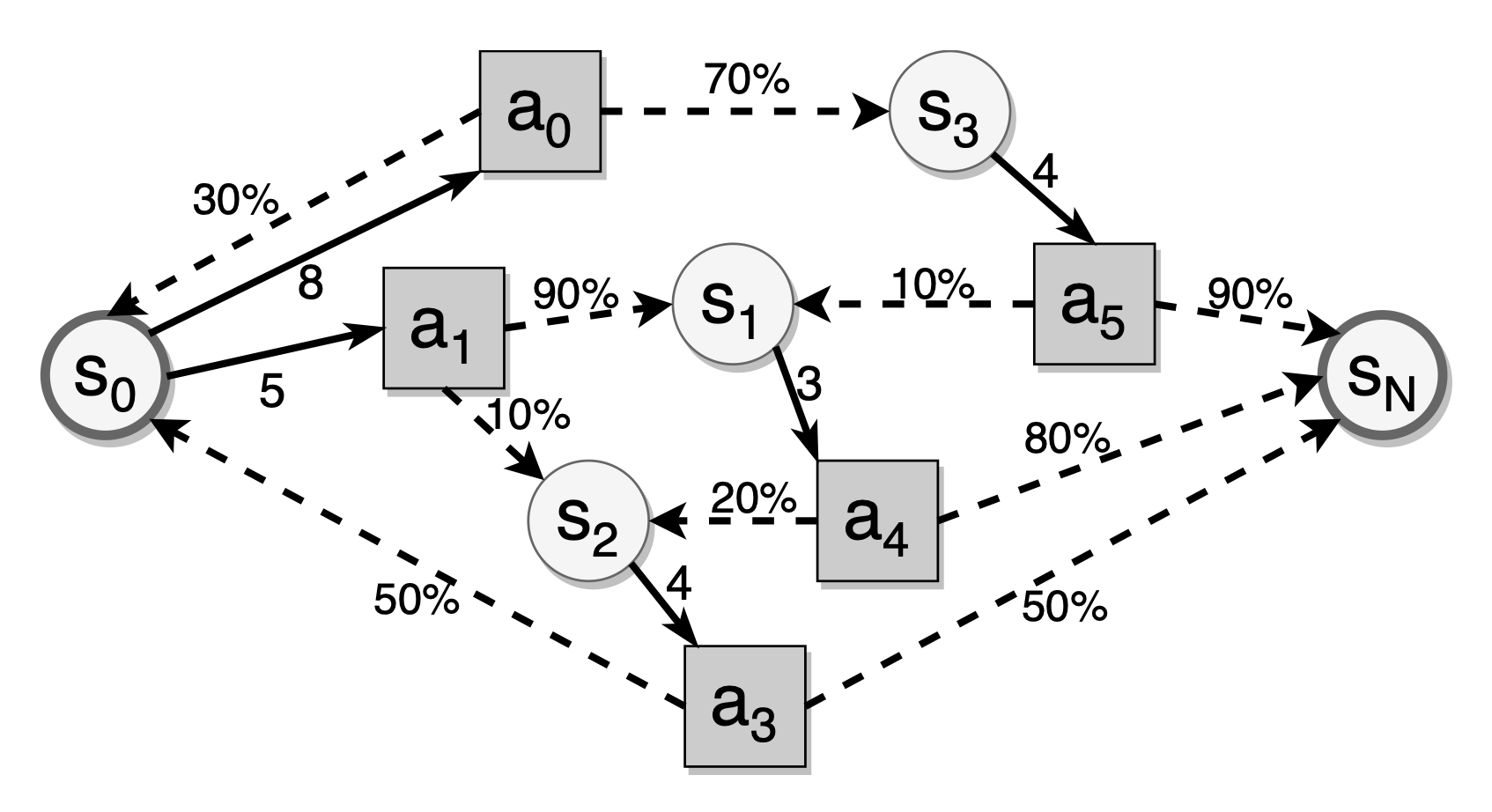
The DSR model satisfies the Markov property. In DSR model, the state of each memory depends only on the last stability, the difficulty, the current review interval, and the result of the recall, which follows a random distribution relying on the review interval. Due to the randomness of stability state-transition, the number of reviews required for mem- orizing material to reach the target stability is uncertain. Therefore, the spaced repetition scheduling problem can be regarded as an infinite-time stochastic dynamic programming problem. In the case of forming the long-term memory, the problem has a termination state which is the target stability. So it is a Stochastic Shortest Path (SSP) problem.

As shown in above figure, circles are memory states, squares are review action (i.e., the interval after the current review), dashed arrows indicate state transitions for a given review interval, and black edges represent review intervals avail- able in a given memory state. The stochastic shortest path problem in spaced repetition is to find the optimal review interval to minimize the expected review cost of reaching the target state.

Formulation

To solve the problem, we can model the review process for each flashcard as a Markov Decision Process (MDP) with a set of states $\mathcal{S}$, actions $\mathcal{A}$, state-transition probabilities $\mathcal{P}$, and a cost function $\mathcal{J}$. The aim of the algorithm is to find a policy $\pi$ that minimizes the expected review cost for reaching the target state $s_N$.

$$ \pi^* = \underset{\pi \in \Pi}{\text{argmin}} \lim_{{N \to \infty}} \mathbb{E}{s{0}, a_{0}, \ldots} \left[ \sum_{t=0}^{N} \mathcal{J}(s_{t}, a_{t}) \mid \pi \right] $$

The state-space $S$ depends on the state size of the memory model. In the DSR, there are merely two state variables, thus the state can be formulated as $ s = (D, S) $. The action space $\mathcal{A} = {\Delta t_1, \Delta t_2, \ldots, \Delta t_n }$ consists of $N$ intervals that can be scheduled. The state transition probability $\mathcal{P}_{s,a}(s')$ represents the likelihood of a flashcard being recalled under state $s$ and action $a$. The cost function $\mathcal{J}$ is defined as:

$$ \begin{aligned} \mathcal{J}(s_0) &= \lim_{{N \to \infty}} \mathbb{E} \left[ \sum_{{t=0}}^{N-1} g_t(s_t, a_t(s_t), r_t) \right] \\ r_t &\sim \text{Bernoulli}(p_t) \end{aligned} $$

where the $g_t$ is the cost per stage and the $r_t$ is the result of recall which follows the Bernoulli distribution. The target state $s_N$ corresponds to the desired level of memory stability.

Algorithm

We solve the Markov Decision Process $\text{MDP}(\mathcal{S}, \mathcal{A}, \mathcal{P}, \mathcal{J})$, using value iteration method. The Bellman equation is:

$$ \begin{aligned} \mathcal{J}^(s) &= \min_{a \in \mathcal{A}(s)} \left[ \sum_{s'} \mathcal{P}_{s,a}(s') \left( g(r) + \mathcal{J}^(s') \right) \right] \ s' &= \mathcal{F}(s,a,r,p) \end{aligned} $$

where the $\mathcal{J}^*$ is the optimal cost function, and $\mathcal{F}$ represents the state transition function, specifically within the context of the DSR model. For the sake of simplicity, we only consider the response of recall: $g(r) = a \cdot r + b \cdot (1-r)$, where $a$ is the cost of successful recall and $b$ is the cost of failed recall.

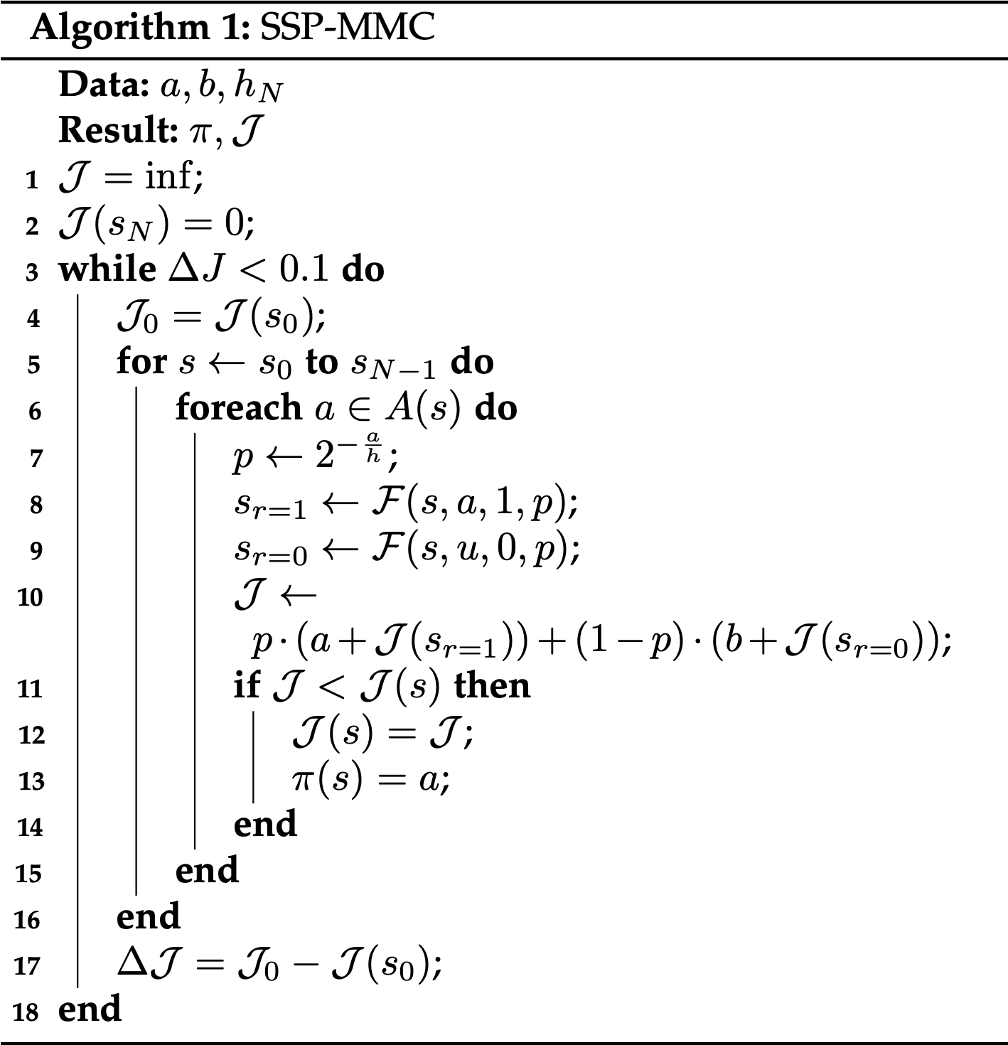
Based on above Bellman equation, the Value Iteration algorithm uses a cost matrix to record the optimal cost and a policy matrix to save the optimal action for each state during the iteration.

Continuously iterate through each optional review interval for each memory state, compare the expected memory cost after selecting the current review interval with the memory cost in the cost matrix, and if the cost of the current review interval is lower, update the corresponding cost matrix and policy matrix. Eventually, the optimal intervals and costs for all memory states will converge.

In this way, we obtain the optimal review policy. Combined with the DSR model for predicting memory states, we can arrange the most efficient review schedule for each learner using the SSP-MMC algorithm.

This algorithm has been open-sourced in MaiMemo's GitHub repository: maimemo/SSP-MMC: A Stochastic Shortest Path Algorithm for Optimizing Spaced Repetition Scheduling (github.com). Readers interested in an in-depth examination are encouraged to fork a copy for local exploration.

Conclusion

Congratulations on reaching the end! If you haven't given up, you've already entered the world of spaced repetition algorithms!

You may still have many questions, some of which may have answers, but many more are unexplored areas.

My capacity to address these questions is decidedly limited, yet I am committed to dedicating a lifetime to advancing the frontiers of spaced repetition algorithms.

I invite you to join me in unraveling the mystery of memory. Are you willing to walk this path with me?

References

History of spaced repetition - supermemo.guru

A Stochastic Shortest Path Algorithm for Optimizing Spaced Repetition Scheduling | Proceedings of the 28th ACM SIGKDD Conference on Knowledge Discovery and Data Mining

Optimizing Spaced Repetition Schedule by Capturing the Dynamics of Memory | IEEE Journals & Magazine | IEEE Xplore

---

Original link: https://l-m-sherlock.github.io/thoughts-memo/post/srs_algorithm_introduction/