google-sheets.md

Google Sheets

Range

• Range in Google Sheets

  What is a range?

  • A range represents a single cell or a group of ADJACENT cells in your spreadsheet. Every time you work with data in a spreadsheet, you're likely using one or more ranges.

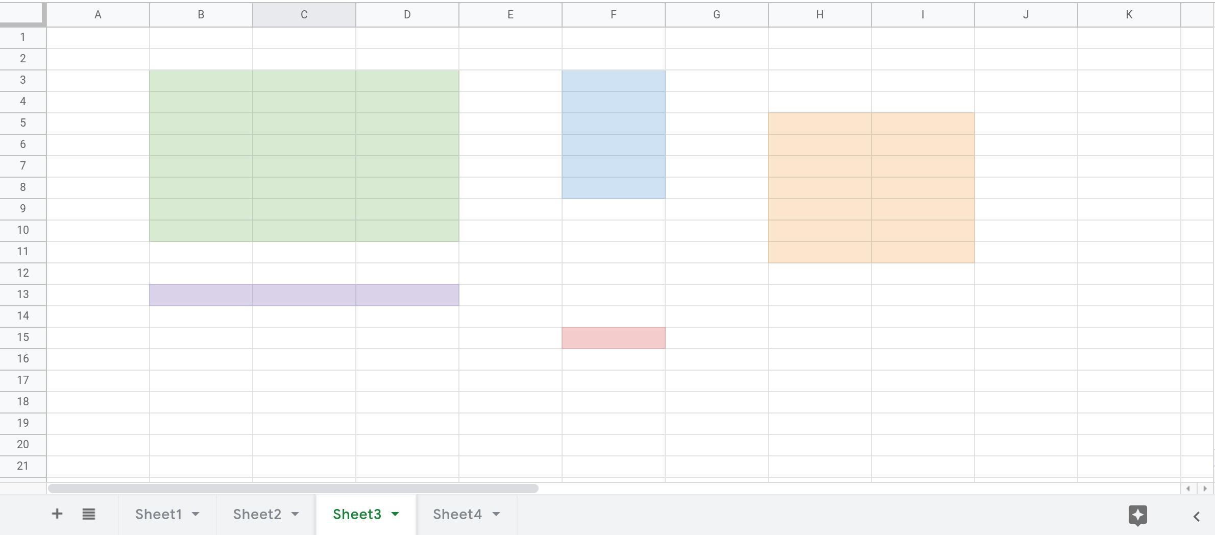
    The screenshot below shows 5 different ranges in Sheet3 of your spreadsheet.

    

  How to reference a range in a Google Sheets formula?

  • To reference a single cell in a formula, use the name of the sheet followed by an EXCLAMATION MARK, the column and finally the row.

    A cell that is in Sheet1 at the intersection of column C and row 5 will have the following reference: Sheet1!C5. This type of reference is known as A1 NOTATION.

  • To reference a range composed of a group of adjacent cells, we'll need to specify the two cells that are at corners of any DIAGONAL within the range. Typically, the cells that are at the top left and bottom right corner are the ones that are specified.

    If the group of cells is fully contained within a single row or column then the top left and bottom right cells are just the first and last cells in the group. ??

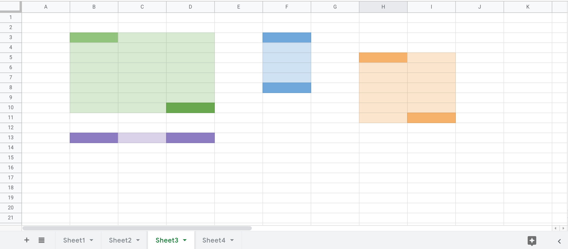
  • The screenshot below displays multiple ranges (the ones that have been colored) and in each case the top left and bottom right cells have been filled with a darker color.

    

    To reference a group of cells in a formula, use the name of the sheet followed by an exclamation mark, the column of the top left cell, its row, a colon, the row of the bottom right cell and finally its column.

    For example, the below references correspond to the ranges highlighted in the above screenshot.

    • Range colored green: Sheet3!B3:D10
    • Range colored blue: Sheet3!F3:F8
    • Range colored purple: Sheet!B13:D13
    • Range colored orange: Sheet3!H5:I11

  • You can also define ranges that reference ENTIRE ROWS OR COLUMNS:

    • All rows in one column: Sheet3!B:B (use the column name twice and omit the row numbers)
    • All rows in multiple adjacent columns: Sheet3!B:D (use the names of the first and last column in the range and omit the row numbers)
    • All columns in a single row: Sheet3!2:2 (use the row number twice and omit the column names)
    • All columns in multiple adjacent rows: Sheet3!2:10 (use the numbers of the first and last row in the range and omit the column names)

  How to use a range in a Google Sheets function?

  • To use a range in a function, just use the range's reference. For example, in order to calculate the sum of values in the range Sheet4!D2:E6, use the formula =SUM(Sheet4!D2:E6). To sum values in just a single cell, say Sheet4!B2, use =SUM(Sheet4!B2).

• Name a range of cells - Computer - Docs Editors Help

  • You can name ranges in Google Sheets to keep better track of them and create cleaner formulas.

    For example, instead of using "A1:B2" to describe a range of cells, you could name the range "budget_total." This way, a formula like "=SUM(A1:B2, D4:E6)" could be written as "=SUM(budget_total, quarter2)."

Dollar Sign

• Cell References and Using the Dollar Sign

  • A formula in a cell in Google Sheets often contains references to other cells in the sheet. A reference to a single cell is a combination of a letter and a number. For example, A1, C5, and E9 are all references to a single cell. The letter indicates the column and the number indicates the row.

    A range is referenced by using two cell references separated by a colon. Ranges can span multiple rows and/or columns. For example, A1:A6 means all the cells in column A from row 1 to row 6, C1:E1 means all the cells in row 1 from column C to column E, and C3:D6 means all the cells in columns C and D from row 3 to row 6. These ranges are shown in the figure below.

  • When a cell containing a formula is copied and pasted into another cell, or if the cell is used to autofill a range of cells, the references in the formula are UPDATED AUTOMATICALLY In each of the new cells.

    Each reference is updated so that the cell it points to is located the same number of rows and columns away from the cell containing the formula as in the original case. So if the formula “=2*A1” is entered into cell B1 and copied into cells B2, B3, and B4, the formula will be changed as shown in the figure below. EACH FORMULA REFERS TO THE CELL IMMEDIATELY TO ITS LEFT.

    

  • A dollar sign ($) can be used before the column and/or row part of a reference to control how the reference will be updated. The dollar sign causes the corresponding part of the reference to REMAIN UNCHANGED. As an example, if the formula “=A$1+$B1” is entered into cell C1 and then copied into the rest of the cells in C1:D4, the resulting formulas will be as shown in the figure below.

    

    注意 C1 (A$1+$B1) 往 C2 複製時，理當變成 A2+B2，但因為 $ 的關係，變成 A$1+$B2；往 B1 複製時，理當變成 B1+C1，結果也因為 $ 的關係，變成 B$1+$B1；也就是 $ 有 remain unchanged 或 lock 的效果。

Conditional Formatting

• 要先瞭解含有 $ 的 formula 被複製到其他 cell 的效果 (remain unchanged / lock)，因為 conditional formatting 搭配 custom formula 使用時，可以想成是把設定值複製到 range 內的所有 cell。
• 搭配 custom formula 使用時，只能參照同一個 sheet 的 cell，否則會出現 "Conditional format rule cannot reference a different sheet." 的錯誤訊息。

參考資料：

• How To Apply Conditional Formatting Across An Entire Row In Google Sheets

  • Conditional formatting is a super useful technique for formatting cells in your Google Sheets based on whether they meet certain conditions.

    For example, you could use it to apply background colors to cells based on the value in the cell.

  • You can go further than this though, and apply the formatting across an entire row, based on the value in a single cell.

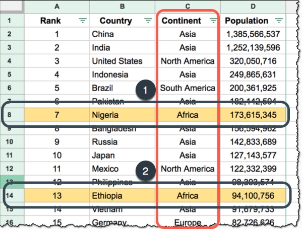
    For example, if the continent is “Africa” in column C, you can apply the background formatting to the entire row (as shown by 1 and 2):

    

  Five steps to apply conditional formatting across an entire row

  • It’s actually relatively straightforward once you know the technique using the $ sign (Step 5).

  • Step 1. Highlight the data range you want to format

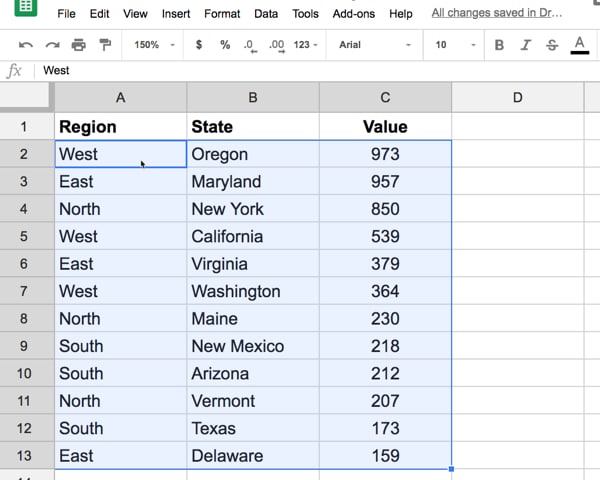
    The first step is to highlight the range of data that you want to apply your conditional formatting to. In this case, I’ve selected: A2:C13

    

  • Step 2. Choose Format > Conditional formatting… in the top menu

    Open the conditional format editing side-pane, shown in this image, by choosing Format > Conditional formatting… from the top menu:

  • Step 3. Choose “Custom formula is” rule

    Google Sheets will default to applying the “Cell is not empty” rule, but we don’t want this here.

    Click on the “Cell is not empty” to open the drop-down menu:

    Scroll down to the end of the items in the drop-down list and choose “Custom formula is”. This will add a new input box in the Format cells if section of your editor:

  • Step 4. Enter your formula, using the $ sign to LOCK YOUR COLUMN REFERENCE

    In this example, I want to highlight all the rows of data that have “West” in column A. In this new input box, enter the custom formula: = $A2 = "West"

    The key point to understand is that you LOCK THE COLUMN YOU WANT TO BASE your conditional formatting on by adding a $ (dollar sign) to the column reference.

    I start inputting the first cell of my highlighted range: = A2

    Then I add the $ (dollar sign) in front of the A only: = $A2

    Then I add the TEST CONDITION, in this case whether the cell equals “West”: = $A2 = "West"

    As the conditional formatting test is APPLIED ACROSS EACH ROW, the value from the first cell in column A is used in the check.

  More examples of conditional formatting across an entire row

  • Based on a threshold value

    This is a super useful application of this technique, to dynamically highlight rows of data in your tables where a value exceeds some threshold.

    In this example, I’ve highlighted all of the students who scored less than 60 in class, using this formula in the custom formula field: = $C2 < 60

  • Based on checkboxes

    Google Sheets checkboxes are super useful. If you haven't heard of them or used them yet, you're missing out.

    When a checkbox is selected it has the value TRUE, and when it is not selected the cell has the value FALSE. So we can use that property in our custom formula: = $B2 = TRUE

Filter

• Filter data in a spreadsheet - Google Workspace Learning Center

  • If you're looking at a spreadsheet with other people, create a filter view that ONLY CHANGES YOUR VIEW of the data.

  • Working with collaborators on the same spreadsheet? Because filter views are turned on by each person viewing a spreadsheet, use a filter view to filter data WITHOUT CHANGING HOW OTHERS SEE the spreadsheet.

  • Share different filter view LINKS with different people, so each person sees the most RELEVANT information.

    切換 filter view 後，URL 會帶有 fvid 參數。

  • Save and name multiple filter views for quick access and sorting later.

  • Make a copy or create another view with similar rules.

  • Don’t have edit access to a spreadsheet and still want to filter or sort? Create a TEMPORARY FILTER VIEW.

    因為 filter 會影響到其他人的關係，所以要有編輯權限；但 filter view 不是會與他人共享嗎??

  Filter data without changing what collaborators see

  1. In Google Sheets, open the spreadsheet where you want to create a filter view.

  2. Click a cell that has data.

     選擇 cell 跟 filter view 的 range 是什麼關係??

  3. Select Data > Filter views > Create new filter view.

  4. Click a drop-down list in a column header and select the data you want to filter. Your filter view is saved as you make changes.

  5. (Optional) To search for data, enter text in the search box.

  6. After you select the data to filter, click OK.

  7. Repeat steps 4–6 for each column you need to filter.

  8. In the Name box, enter a name for your filter view. If you don’t enter a name, the filter view is saved as Filter number, where number corresponds to the number of filters you’ve created.

     Your saved filter view now appears in Data > Filter views. Filter views have DARK GRAY HIGHLIGHTS in the column and row headers.

  Filter data for everyone

  1. Select a range of cells.
  2. Click Data > Create a filter.
  3. Go to the top of the range and click Filter to see the filter options.

參考資料 {: #reference }

手冊：

• Keyboard shortcuts for Google Sheets